Next Generation Sequencing (NGS) technologies have increased exponentially the understanding of the genomic structure and function of different organisms within the last decade, including the CIAT mandate crops. In order to handle the vast amount of data produced by these technologies, several bioinformatics tools have been developed to carry on different kinds of analysis. However, most of these tools are not easy to operate, integrate and customize without the technical support of experts in bioinformatics, which produces a bottleneck for several research efforts. This situation sets the need for integrated data analysis pipelines with user friendly interfaces available to the scientific community.

We have developed NGSEP (NGSTools Eclipse Plugin), an integrated framework for variants discovery from NGS data. NGSEP is based on Eclipse which is one of the leading development environments for Java. We integrated previously developed algorithms for SNV detection available in the NGSTools package with Java implementations of state-of-the-art algorithms for CNV and structural variation discovery. NGSEP provides an intuitive interface in which the user has a rich control over the files produced during the different stages of the analysis. These files follow current standard formats such as BAM and VCF, which makes NGSEP results easy to integrate with genome visualization tools. NGSEP can also be integrated with bowtie2 to allow the user to follow all the steps needed to obtain genomic variants from raw reads without scripting. NGSEP will be distributed as an open source project under General Public License (GPL) to make it available to the scientific community.

System Requirements

In order to install and execute NGSEP plugin properly you must have installed the following components:

-Operative system Windows, Macintosh or Linux.

- Java (jre jdk 1.6 or higher). See instructions for how to check your current version of java or download it and install it, in page 4.

- Eclipse IDE 3.7 or higher. See instructions for how to download and install Eclipse in page 5.

- Bowtie2 is required only for the Map Reads function. See instructions for how to download and install Bowtie2 in the section Map Reads on page 16.

-WinRar or WinZip.

-Text editor. We recommend notepad++. You can download it in the following link: http://notepad-plus-plus.org/

Command Line

You can also run NGSEP from the command line, downloading the NGSEP library: NGSToolsApp.jar from http://sourceforge.net/projects/ngsep/files/Library/. Look at the README file for instructions on how to run the command line version of NGSEP.

Downloading and Installing Java

NGSEP is written in Java and therefore platform independent, but the Java Runtime Environment (JRE) version 1.6 or higher (also called Java 6) has to be installed. You can check the version of your Java JRE, and test if it is working, using the following link:

http://www.javatester.org/version.html

Downloading Java for Windows

To Download and install Java6 RE from the following link: http://www.oracle.com/technetwork/java/javase/downloads/index.html

Downloading Java for Mac

Apple Computer supplies their version of Java. Use the Software Update feature (available on the Apple menu) to check that you have the most up-to-date version of Java for your Mac. Additionally, make sure that Java version 1.6 is set as first preference version. This can be changed under "Applications - Utilities - Java Preferences.app". You can also download the Mac OS X x64 Option from http://www.oracle.com/technetwork/es/java/javase/downloads/jre7-downloads-1880261.html

Downloading and Installing Eclipse IDE

For 64 bit operating system

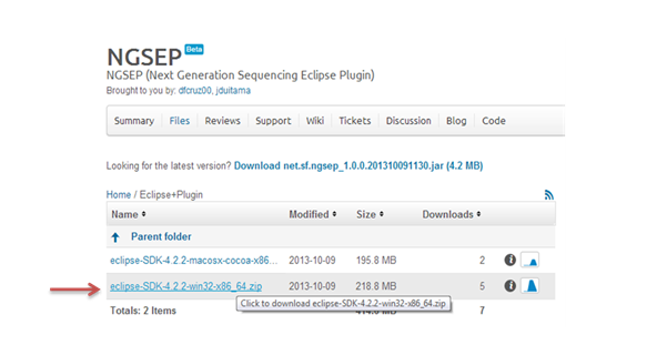
We offer the option to download the latest release of Eclipse IDE together with NGSEP plugin and a Bowtie2 auto installer for Windows “Eclipse+Plugin”. However, this option is only available for 64 bit operating systems.

Select the “Eclipse+Plugin” option, and then the adequate .zip file according your operative system. Unzip the file clicking the option extract into your work folder.

In the extracted folder called eclipse, you will find a folder called “dropins”. In this folder you will find the NGSEP plugin.

In addition, you will find the executable file for eclipse (eclipse.exe). Click in this file to launch eclipse. It will immediately ask you for a work folder called workspace. You can select the suggested one or assign a specific one. This will be you working folder in Eclipse, where all your projects are going to be created. Now eclipse is ready to be used.

For 32 bit operating system

If you are using a 32 bit operating system, download first the standard Eclipse (http://www.eclipse.org/downloads/) for 32 bit and then download the NGSEP plugin “OnlyPlugin” (https://sourceforge.net/projects/ngsep/files/OnlyPlugin/). Follow this instructions on how to download and install the NGSEP plugin and eclipse:

Select the “OnlyPlugin” option.

Download the compressed file from the download page of eclipse organization: http://www.eclipse.org/downloads/ .

Select Eclipse Standard 4.3.1 and choose the right file according to your operative system and your system architecture (32 or 64 bits).

Unzip the file clicking the option extract into your work folder.

In the extracted folder you will find an executable file called eclipse.exe: Once you click on that file, eclipse will be launched and immediately it will ask you for a work folder called workspace. You can select the suggested one or assign a specific one, this will be you working folder in Eclipse, where all your projects are going to be created. Now eclipse is ready to be used.

Eclipse will look for your java virtual machine (JVM). If it is not recognized please follow the next directions:

Once installed, you must edit the PATH variables. In windows you can access them trough: MY PC – PROPERTIES – ADVANCED OPTIONS – ENVIRONMENT VARIABLES

Click on environment variables, search for PATH Variable and edit it adding a “ ; “ plus the path for the \bin folder from the JVM at the end of the line (where you can find the executable files of the JVM), for example:

“; C:\Program Files\Java\jre1.6.0_20\bin “

Restart your PC so that the change will be applied, and Java will be available for all the system and therefore for eclipse.

Increasing eclipse memory

It is highly recommended to increase the values of memory granted for eclipse because NGSEP runs processes which are demanding, producing exceptions in some functionalities when there is not enough memory assigned to eclipse. The most common error that reflects this issue would be Exception in thread “main” java.lang.OutOfMemoryError: Java heap space. In order to be able to increase these values of memory, locate eclipse folder and edit a file called eclipse.ini, which looks like something like the following picture:

Note: Before editing this file, make sure that eclipse is closed; otherwise the changes will not be applied.

Inside that file, you will find the line –Xmx___m

This line indicates how much memory eclipse is allowed to use. In this example we set Xmx3500m. It is recommended to use 3 Gb if your RAM memory is higher than 6 Gb otherwise you can try with 1500mb or start decreasing until the eclipse launch successfully.

Save and close the file and launch again the eclipse.

Note1: You can check your RAM memory in Control Panel à All Control Panel Items à Systems.

Note: The eclipse.ini file, is often hidden in your eclipse folder. To unhide this file, go to Control Panel à Folder Options à View tab and select the “Show hidden files, folders and drives option. Also it is recommended to unselect the option “Hide extensions from known file types” to be able to recognize the files by the extension.

NGSEP download, installation and use

To install the NGSEP, you need to download NGSEP plugin (http://sourceforge.net/projects/ngsep/files/OnlyPlugin/) and paste the in a folder called dropins in the eclipse directory. If you download the “Eclipse+Plugin” version for 64 bits, the plugin comes already in the dropins folder in eclipse.

After restarting eclipse again, the NGSEP plugin will be integrated with eclipse IDE.

NGSEP update

To update NGSEP, download the latest version of the plugin from the web site (http://sourceforge.net/projects/ngsep/files/OnlyPlugin/). Erase and replace the new version in the dropin folder in the eclipse directory. Restart eclipse and the NGSEP plugin will now be integrated with eclipse IDE.

Create a new project

The first thing that you need to do after starting eclipse is to create a new project. To create a new project, go to the task bar at the upper part of eclipse, and select: File àNew Project, and choose General à Project. Immediately a window to name the project will show up, where you can type the name of your new project.

Upload Files

The standard input files could be in BAM, SAM, FASTA or FASTQ formats, depending of the kind of analysis you want to perform:

To add your input files to the project you just created, select the group of files from their corresponding directories, then copy and paste them or drag them directly in your project in eclipse.

Once you pasted the selected files, you can view them on the project in eclipse as shown in the following image.

We suggest creating folders according to the type of data they contain, for example folders for the references, the raw reads etc., as follows:

Now NGSEP should be working in your eclipse. If you do right click on any input file, for example the .Bam, you will see several options, and you should be able to locate NGSEP among them. If you put the mouse cursor on it, you will see the bioinformatics options that NGSEP can execute, from map reads to variants detection and statistics plots.

Note: Remember to always refresh your project folder after running any process to enable to see and update your output and .log files. Press F5 or by make right click at your project folder and select the option refresh.

Tracking Process Progress

Enable NGSEP Progress Bar

Enabling the NGSEP view in eclipse, will allow you to see the progress bar of the NGSEP tasks.

To enable the progress bar, go to the tools bar at the upper part of eclipse and select the following options:

Windows à Show viewàOtheràNGSEPView

Note: you could find some differences among Eclipse versions.

Remember, you have to paste the plugin in the dropins folder; otherwise the progress bar will not be displayed.

1. First click on window option in the task bar.

2. Then click on the option Show view àOther.

3. Click on the folder General and choose NGSEPView

4. You will be able to see a new tab next to the console and problems log.

Note: This tab contains the progress bars of NGSEP. If you haven’t triggered any process you should not see anything there, however sometimes eclipse uses that tab to report processes of projects and its environment. Do not worry if that happens. Now with the progress bar view activated you are ready to use the different options that NGSEP offers.

Error and process tracking

To check if your process in NGSEP were successfully completed, you can check the .log files, generated by each function. The name of the log file will have the prefix of the executed process, followed by the output name and the .log extension. You can check this file at any point of the process, and it will contain information on the progress of your process, or information about any possible error.

You can find your .log files, in your project folder, directly in eclipse.

Note: Remember to refresh your project folder frequently using F5 or by making right click at your project folder and select the option refresh.

Another source of error, independent of NGSEP could be tracked by looking at eclipse’s error log file. There are two ways to check this log file. First, you can enable the error view in eclipse, selecting Window à Show View à Error log.

Second, you can find a .log file in a folder called .metadata, located in: workspace_folder/.metadata/.log. You can open it with your default text editor and check for any possible errors. This could be useful anytime that the source of error do not allow to open eclipse.

Note: Usually the .metadata folder could be hidden. In this case, you should enable to look for hidden files and folders.

Map Reads

This process executes the alignment or mapping process between a reference genome and reads that come from sequencers such as Illumina and 454. This process can be performed for a single sample or for multiple samples (see Multi Map Reads).

REQUIREMENTS

— Bowtie2: Open source tool that is able to map up to 25 million of short reads (35 pb) per hour.

Installing Bowtie2

The first step to use Map reads is downloading and installing bowtie2 in your PC. In NGSEP we provide a bowtie2 auto installer for Windows operating systems of 64 bits, which makes easier the installation process. You can find the auto installer in the folder Elipse+Plugin in http://sourceforge.net/projects/ngsep/files/Eclipse%2BPlugin/. This auto installer was created using Advanced Installer version 10.6 http://www.advancedinstaller.com.

Download the .zip adequate for your operating system, unzip it and you will find a folder named “InstallBowtie2”. To install bowtie 2 using the auto installer, double click on the Bowtie2.msi link.

Follow the default options, until installation is complete.

To check whether bowtie2 was successfully installed, we recommend the following test:

Look for the cmd command line in Windows, by typing cmd in the search bar.

Then type bowtie2-align.exe in the command line, and you should be able to see all the options available for bowtie2 as in the following screen:

If Bowtie2 was not successfully installed, then after this test you should have the following message:

For a manual installation of bowtie2, if for instance you have a 32bits Windows operation system, follow these instructions:

Download Bowtie2

1. Download Bowtie2 in the following link: http://sourceforge.net/projects/bowtie-bio/files/bowtie2/2.1.0/ and extract the code to a location on your disk.

2. Find the executable: bowtie2-align.exe, bowtie2-build.exe.

3. Add bowtie2 to your PATH environment variable. To do this, follow your operation system’s instructions for adding the directory to your Path. For Windows follow these steps:

A. Make a right click on Computer and choose: Properties à Advanced System Settings à Advanced Options à System Variables àPath à Edit. In the option Variable Value, add a “;” (each semicolon adds a new path for variables) and write the path where your bowtie2 folder is.

B. For example:

C. ;C:\Users\jcqui02ntero\Desktop\CIAT\Bowtie2\bowtie2-2.1.0\bowtie2-align.exe

Index of the reference with Bowtie2

To perform the Map reads function you will also need an index for the reference genome; otherwise the process will not start.

NGSEP provides an easy way to generate an index of your reference genome, using Bowtie2:

First, you need to upload your reference file in FASTA format (.fa ) in eclipse. Make a right click in the file and select the “Create Index Bowtie” function in the NGSEP menu. An option will pop-up that by default will recognize and show your input file ( (*)Reference) and the name and pathway of your output file, that by default will be the same as the reference ((*)Index Bowtie2 Prefix). Here you can change the input reference file, the output prefix, or both, using the browsing option at the right.

For more information about the indexing process in bowtie2, we recommend these links:

http://bowtie-bio.sourceforge.net/bowtie2/manual.shtml

http://sauron.cs.umd.edu/bowtie2/doc/manual.html - the-bowtie2-build-indexer

Using Map Reads

After completion of the index of the reference genome, you can execute the Map Reads function in NGSEP. (Through this entire manual we are going to use as example for mapping input files, Illumina Fastq formats. However, other file formats are also allowed).

You will need your input files in FASTQ format (.fq or .fastq) uploaded in your eclipse IE.

You can select a unique file or two files in case that you have complementary data. Make right click in the file/s and select the Map Reads function in the NGSEP menu.

Choose the adequate parameters (explained below) for your analysis:

Map Reads parameters

The parameters described below are summarized from the parameters of alignment in Bowtie2 that you can find more detailed in Bowtie2 manual, at Bowtie2 official page (http://bowtie-bio.sourceforge.net/bowtie2/manual.shtml).

Input and Output Files

File #1 y File #2 fields show the path of your input files. To change your input files use the browser option.

(*)Index Bowtie2: Select the reference index (can be created using Create Index Bowtie option previously described). Next time that you open this screen you will see the last file that you upload.

(*)Output File (.bam): Enter the name and the path where you want to save your output file. The name of the file must end with the extension .bam

Input

Select the Input flag if you know the format of your input files, and choose the adequate option. If you don’t select the Input file format, the program will assume FastQ as default.

The different file formats are listed the chart below. For a complete description we recommend the following link:

http://www.ncbi.nlm.nih.gov/books/NBK47537/

Input File Format
Fasta	FASTA files usually have extension .fa, .fasta, .mfa, .fna or similar. A sequence in FASTA format begins with a single-line description, followed by lines of sequence data. The description line is distinguished from the sequence data by a greater-than (">") symbol in the first column. The word following the ">" symbol is the identifier of the sequence, and the rest of the line is the description (both are optional).
FastaQ	FASTQ files usually have extension .fq or .fastq. This is the default format. This format is similar to fasta consisting of readname headers, nucleotide base calls and per-base quality scores in text form. Illumina fastq contains the READNAME, index, read number parameters with quality basis character @. Paired end data are presented in the orientation in which they will be aligned to a reference (5’-3’-3’-5’), which is the same orientation they were sequenced in.
Ilumina qseq format:	This format is similar to FASTQ but differs in how the quality scores are calculated. QSEQ files usually end in _qseq.txt.
Raw one-sequence-per-line:	Reads are files with one input sequence per line, without any other information (no read names, no qualities).

Phred

This option allows for choosing between the Phred+64 and Phred+33 encoding formats. If you don’t select the phred64 option, default will be phred33.

Trim

With this option you can trim low quality bases from the 5' and/or 3' end of each read. Low quality bases could be detected using the quality statistic option describe in Quality Statistics.

Trim5’: Number of bases you want to remove from 5' (left) end of each read before alignment (default: 0).

Trim3’: Number of bases you want to remove from 3' (right) end of each read before alignment (default: 0).

Read Group data

In Read group Id enter a tag that is going to be used for the output bam files for further classifications/grouping of the samples.

Reporting

The reporting mode allows for the search for one or more alignments and to report each one. Bowtie2 has three distinct reporting modes. The default mode is similar to the default reporting mode of many other read alignment tools, including BWA. It is also similar to Bowtie 1's -M alignment mode. In general, for this option when a read has an alignment, it means that it has a valid alignment. When it has multiple alignments, it means it has multiple alignments that are valid and distinct from one another.

If you choose Numbers of Alignments to report, you will find another field available where you can input the number of alignments you want to report.

Using this option, Bowtie 2 searches for as many valid alignments for each read as you specify in the “Number of Alignments to report” field. If, for example, you choose 2, Bowtie2 will search for at most 2 distinct alignments. It reports all alignments found, in descending order by alignment score. The alignment score for a paired-end alignment equals the sum of the alignment scores of the individual mates.

Bowtie 2 does not "find" alignments in any specific order, so for reads that have more than N distinct, valid alignments, Bowtie 2 does not guarantee that the N alignments reported are the best possible in terms of alignment score. Still, this mode can be effective and fast in situations where the user cares more about whether a read aligns (or aligns a certain number of times) than where exactly it originated.

Effort

In the Give up extending after option you can choose the number of consecutive seed extension attempts that can "fail" before Bowtie 2 moves on, using the alignments found so far. A seed extension can fail if it does not yield a new best or a new second-best alignment. Default value is 15.

With the Maximum number of times for re-seed option you can choose the maximum number of times Bowtie 2 will "re-seed" reads with repetitive seeds. When "re-seeding," Bowtie 2 simply chooses a new set of reads (same length, same number of mismatches allowed) at different offsets and searches for more alignments. A read is considered to have repetitive seeds if the total number of seed hits divided by the number of seeds that aligned at least once is greater than 300. In this case, the default value is 2.

Alignment

With the option Length of seed substring you can set the length of the seed substrings to align during multiseed alignment. Smaller values make alignment slower but more sensitive. Default value is 20.

Interval beteen seed substrings sets a function governing the interval between seed substrings to use during multiseed alignment. For instance, if the read has 30 characters, and seed length is 10, and the seed interval is 6, the seeds extracted will be:

Read: TAGCTACGCTCTACGCTATCATGCATAAAC

Seed 1 fw: TAGCTACGCT

Seed 1 rc: AGCGTAGCTA

Seed 2 fw: CGCTCTACGC

Seed 2 rc: GCGTAGAGCG

Seed 3 fw: ACGCTATCAT

Seed 3 rc: ATGATAGCGT

Seed 4 fw: TCATGCATAA

Seed 4 rc: TTATGCATGA

Since it's best to use longer intervals for longer reads, this parameter sets the interval as a function of the read length, rather than a single one-size-fits-all number. For instance, specifying values of 1, 2.5 sets the interval function f to f(x) = 1 + 2.5 * sqrt(x), where x is the read length. If the function returns a result less than 1, it is rounded up to 1. Default value: 11,0.75.

With this option you can specify the number of positions you want to disallow gaps at the beginning or end of the read. Default value is 4.

This option "Pads" dynamic programming problems by the number of specified columns on either side, to allow gaps. Default value is 15.

This option sets a function governing the maximum number of ambiguous characters (usually Ns and/or .s) allowed in a read as a function of read length. For instance, specifying -L, 0, 0.15 sets the N-ceiling function f to f(x) = 0 + 0.15 * x, where x is the read length. Reads exceeding this ceiling are filtered out. Default values are L, 0, 0.15.

Sets the number of maximum mismatches allowed in a seed alignment during multiseed alignment. It can be set to 0 or 1. Setting this higher makes alignment slower (often much slower) but increases sensitivity. Default value is 0.

When calculating a mismatch penalty, always consider the quality value at the mismatched position to be the highest possible, regardless of the actual value. I.e. input is treated as though all quality values are high. This is also the default behavior when the input doesn't specify quality values

If Nofw is specified, bowtie2 will not attempt to align unpaired reads to the forward (Watson) reference strand. If Norc is specified, bowtie2 will not attempt to align unpaired reads against the reverse-complement (Crick) reference strand. In paired-end mode, Nofw and Norc pertain to the fragments; i.e. specifying Nofw causes bowtie2 to explore only those paired-end configurations corresponding to fragments from the reverse-complement (Crick) strand. Default: both strands enabled.

Paired-end Alignment

In this option you can specify the minimum and maximum fragment length for valid paired-end alignments.

Finally, the Map Reads button is the option that performs the process invoking Bowtie2, after validating the data entered.

Final Results for Map Read:

-At the end of the process you will generate a .Bam file with all the reads matched against the reference.

Multi-Mapping

This process is similar to Map Reads (See Map Reads) but allows performing multiple mappings in parallel, saving time since the execution of the process is divided and executed in parallel into the number of processors you choose.

Likewise, this function has the same requirements as the Map Reads function: to have Bowtie2 installed, and to index your reference genome (See Map Reads).

For this function, you will need to create a new folder or directory in eclipse only with your fastq files, whether they are paired or simple reads. These files need to be uncompressed (i.e If you have a .gz ,.zip, .rar, you need to uncompressed them before upload them in eclipse). Make right click on the directory and select the Map Reads function in the NGSEP menu.

Screen Multi Mapping

The Multi Mapping screen will display your fastq files organized on a table, with each pair of files (in case of complementary data) or simple files in one line. It will recognize paired files by the same name and different prefix. Select and unselect all the files for the mapping process with the option, or individual samples by selecting the check box at the left.

In the Output Directory you can select the path and directory where all your output files are going to be generated; by default is the same directory path where the process was launched.

Exception: To enter the next screen you must select at least one sample the table.

If you want to change any of the files of your current directory, double-click the cell you want to change, and browse the directory path of your new sample.

After choosing Next, you will find another screen with the Map Reads options. Choose the adequate parameters (explained in Map Reads parameters) for your analysis.

Sort Alignment

This option sorts the Bam file. This process is required because sequencers such as Illumina, 454 and Sanger among others, produce files that match randomly in the genome. Sort Alignment uses internally Picards Tools, a library which already contains an option for this purpose. The Map Reads option described above automatically performs the sort alignment of the reads. However, if you start from unsorted Bam files, you must use this option to sort them.

INPUT FILES

· BAM: Text format tab delimited file which consist in a header section, that is optional and a section of alignment. The header begins with @ while the alignment lines don’t. Each aligned line has 11 optional information fields that make it flexible. For a detailed description of a bam file we suggest the following reference (http://samtools.sourceforge.net/SAMv1.pdf) that you can find in the SAM tools web page.

OUTPUT FILES

· SORTED BAM: BAM file organized by chromosome and reference position.

ACCESS TO SORT ALIGNMENT

1. The first step in order to access to Sort Alignment after installing Eclipse and NGSEP is having the Bam file.

2. Click on the .Bam file, and choose the Sort Alignment option from the NGSEP menu.

3. Make sure that you only select one Bam file.

The first field is the File (Bam), which shows the path of the input file that you browsed. The next one is (*) Output file: This text field holds the same input name with the addition of the word “_sorted” just before the extension. Also, you can change the output destiny directory and file name. Our advice is to use the same directory because further processes will require them.

4. Use the button with the label Sort Alignment to execute.

Final Result for Sort Alignment:

-At the end of the process you will see a similar file than the input, but organized and ready to continue with the pipeline.

Variants Detector

This is the main functionality of NGSEP, which using a Bam file against a reference genome to detect different genomic variations such as: Single Nucleotide Polymorphisms (SNPs), Copy Number Variations (CNVs) and Structural Variants (SVs).

INPUT FILES

— Sorted BAM File : The BAM file is a text format tab delimited file which consists in a header section, that is optional and a section of alignment. The header begins with @ while the alignment lines don’t. Each aligned line has 11 optional information fields that make it flexible. For a detailed description of a bam file we suggest the following reference (http://samtools.sourceforge.net/SAMv1.pdf) that you can find in the SAM tools web page. The original bam file needs to be sorted by chromosome and reference position (See Sort Alignment) in order to use the variants detector.

OUTPUT FILES

— VCF (Variant call format): Is flexible and extensible file for variation data such as (SNPs), small INDELs, CNVs and structural variants. For more information of the file format see: http://www.1000genomes.org/wiki/Analysis/Variant%20Call%20Format/vcf-variant-call-format-version-41

— GFF: General format of characteristics created by Sanger, composed by 9 mandatory fields separated by tabs. For more information see: http://www.sanger.ac.uk/resources/software/gff/spec.html

— CNVs format: This file list the detected copy number variations or repeats. It is a file separated by tabs and composed by three columns: the first one is the name of the chromosome/scaffold where the CNV is located. The second and third columns are the start and end positions respectively.

ACCESS TO VARIANTS DETECTOR

1. The first step in order to access to Variants Detector after installing Eclipse and NGSEP is having the Sorted Bam file.

2. Click on the sorted Bam file, and choose the Find Variants option from the NGSEP menu.

3. Make sure that the selected file is a Sorted Bam File otherwise the process will not work.

Screen Variants Detector

Options for Variant Detection

(*)File: In this field you can see the path of the sorted Bam file that you selected (It could be the output file of the Sort Alignment of NGSEP). Note that you can also use the browser on the right in case you want to change the input file.

(*)Reference File: This field is mandatory because the reference genome is going to be used to compare your reads. The first time that you execute this functionality this text field will be blank, you must browse for a fasta file with the reference genome. However, for further executions the field will display the last reference used.

(*)Output File Prefix: This field refers to the output files you will generate with this function. In total you will generate 3 files that will be named with the same output prefix that you type. The generated files will be: VFC: For SNPs and Small indels, CNV: For Copy Number Variations. GFF: For SNVs and large indels. You can change the prefix and the destination directoryof your output file, using the browser on the right.

Notice that the output directory suggested is the same of the input file as well as the name of the tested sample.

Execution Parameters

This section is composed by 4 parameters that represent the whole variant detection process. Select the option you want to skip or avoid from your variants detection process.

-Skip Repetitive Regions Detection: Select this option to avoid the detection of Repetitive Regions for the detection of the other genomic variants.

-Skip New CNV Detection: Select this option to avoid the detection of CNVs for the detection of the other genomic variants.

-Skip SNVs Detection: Select this option to avoid the detection of SNVs or SNPs for the detection of the other genomic variants.

-Skip Structural Variants Detection: Select this option to avoid the detection of structural variants for the detection of the other genomic variants.

Note: If you don’t select any option from Execution Parameters NGSEP will execute all the findings of variants detector.

SNVs Detection Parameters

In this section you will find parameters that can improve the SNVs detection.

Note: Some fields are filled with default values, however if you are aware about their meaning you can change on demand according to your sample on research.

-Genomic Location (optional): In this field, enter a specific location in the genome in order to detect SNPs. This is an example of the format accepted: ‘chr21:33,031,197-33,041,570’.

Note: you must be aware of the number of chromosomes/scaffolds and range of detection.

-Heterozygosity Rate: This field is intended to enter the probability of finding in every certain position an heterozygous SNPs.

-Minimum Genotype Quality Score: Indicate the minimum accepted value of probability to consider an error (Phred Score).

-Maximum Base Quality Score: Maximum score allowed by allele.

-Alternative Allele Coverage: Maximum and minimum number of alleles that can present a position.

-Ignore Lower Case References: Select this option if you want to skip bases in lower case.

-Maximum Alignment Per Start Position: Use this quality filter to allows to correct some errors produced by PCR Amplification Artifacts.

-Known CNVs File: In this file you can enter the path of a CNV file that can be used in you detection.

Common Parameters

This section holds some parameters that are related to all processes in the Variants detection.

-Ploidy: For Haploid type 1, for diploid type 2.

-Sample ID: You can type a specific ID to label the header of the VFC.

Use the button Find Variants to execute

Note: When you execute the variants detector, a progress bar will be displayed on the bottom, it represents the percentage of completed process. This is important because many times this process can takes several minutes depending on how complex is your organism. If you want to stop the process you are able to do it by pressing the red button in the right side of the progress view. At the end of the process you will see the output files in the directory that you selected.

Multi-Variants Detector

This process is similar to Variants Detector (See Variants Detector) but allows performing Variants Detector to multiple samples in parallel, saving time since the execution of the process is divided and executed in parallel into the number of processors you choose.

For this function, you will need to create a new folder or directory in eclipse only with your sorted bam files. Make right click on the directory and select the Multi Variants Detector function in the NGSEP menu.

The Multi Variants Detector screen will display your sorted bam files, each file on a line, organized on a table with the following columns: File One, Sample ID and Output File.

Select and unselect all the files for the finding variants process with the option, or individual samples by selecting the check box at the left.

In the Output Directory you can select the path and directory where all your output files are going to be generated; by default is the same directory path where the process was launched.

Exception: To enter the next screen you must select at least one sample the table.

If you want to change any of the files of your current directory, double-click the cell you want to change, and browse the directory path of your new sample.

Likewise, you can change the sample ID and the output file names by making double-click in the cell you want to change, and entering a new name for these cells in a text box.

In the Output Directory you can select the path and directory where all your output files are going to be generated; by default is the same directory path where the process was launched.

Exception: To enter the next screen you must select at least one sample the table.

After choosing Next, you will find another screen with the Variants Detection options. Choose the adequate parameters (explained in Variants Detection parameters) for your analysis.

Merge VCF

This process is intended to merge variants from different samples into an integrated VCF file. The process is divided in three phases; the first one is intended to determine a list of variants found in at least one of the VCF files that were generated in the variants detection process, generating one common VCF file with the union of variants reported by all the input files but without any genotype information. Afterwards the process requires running again Variants Detector for every sample but using the mentioned common file in the known variants field. This will produce a second set of VCF files which will be different from the first set in the sense that it will include calls to the reference genome. Finally you will be able to join or merge those new individual VCF files in one VCF with all the samples.

ACCESS TO MERGE VCF

1. The first step is making sure that you have the detector variants history file with at least two samples.

2. Click on the file named HistoryFileVCF.ini, and choose the Merge VCF option from the NGSEP menu.

3. Make sure that the selected file is Detector Variants history with more than three samples otherwise the process will not work properly.

(*) Output File: This field means the output file Merge VCF and is mandatory.
Select all files: This option is equivalent to select all rows.
Deselect all files: This option is equivalent to deselect all rows.
Determine list of variants: This option is used to join in one VCF file, without genotypes, all variant alleles found in at least one of the samples or files, without any genotype information.
Merge VCF files: This option is used to join all genomic variants found in the individual VCF files from each sample, into a single VCF file for all samples, matching each corresponding variation with their corresponding genotype in each sample.

An example of the output file using the “Determine list of variants” option looks like this:

The output file is important for the execution of the second process (Merge VCF), because this file is required to execute again variants detector for each sample in order to associate the variant allele with their corresponding sample genotype.

After finishing the list variants process, proceed to right click on each BAM file using the known variants field to run variants detector again as follows:

In the Known Variants File field, you should provide the VCF file you just created above with the first step of Merge VCF.

After running the Variant Detector again for each sample, using the Known Variants File, the output VCF file for each individual sample will look something like this:

After performing this step with the three selected files proceed to click on the List Merge screen, select the new VCF files and click on Merge VCF.

Final Result for Merge VCF:

Finally, the output file after using “Merge VCF” should be a VCF file that includes all the samples, with their corresponding genotypes, and should look like this:

Variants Functional Annotator

This module takes a VCF file produced by NGSEP, the reference genome in fasta format, and a gff3 file with gene annotations related with the given genome (see http://www.sequenceontology.org/gff3.shtml for details) and generates a VCF file which includes the functional information related with each variant.

ACCESS TO VARIANTS FUNCTIONAL ANNOTATOR

1. The first step in order to access to Variants Functional Annotator after installing Eclipse and NGSEP is having the VCF file (It could be the output of the Variant Detector).

2. Click on the VCF file, and choose the Variants functional annotator option from the NGSEP

3. Make sure that the selected file is a VCF File otherwise the process will not work.

Screen for Variants Functional Annotation

4. (*VCF) Variants File: In this field you can see the path of the VCF file that you selected (It could be the output file of the “Variants Detector” function. You can also use the browser on the right in case you want to change the input file.

5. (*)Gene Annotation File: This field is mandatory because it is the basic input of annotations. At the beginning it will be blank; you have to browse a GFF file with the sample annotations. For further executions the field will display the last file used.

6. (*Fasta)Genome Reference: This field is mandatory because the reference genome is going to be used to compare your data. The first time that you execute this functionality this text field will be blank, you must browse for a fasta file with the genome reference. For further executions the field will display the last reference used.

7. (*VCF)Output File: In this field you should enter the name and path where you want your output file; we recommend using the same project directory.

8. Use the button with the label Variants Functional Annotator to execute if you want to close the window click on cancel.

Final Result for Variants Functional Annotator:

-At the end of this process you will see a VCF file holding the information about genes changes and their variations.

Quality Statistics

This process compares the reads held in the .Bam file according to the reference genome, and then NGSEP will be able to indicate the number of sequencing errors for each position of the reads as one set. It should have a homogenous distribution around one.

ACCESS TO QUALITY STATISTICS

1. The first step in order to access to Calculate Quality Statistics after installing Eclipse and NGSEP is having the Sorted Bam file.

2. Click on the sorted.bam file, and choose the Calculate Quality Statistics option from the NGSEP menu

3. Make sure that the selected file is a Sorted Bam File otherwise the process will not work.

Screen Calculate Quality Statistics

4. This screen is composed by 5 field:

File: In this field you can see the path of the input file that you selected (It could be the output file of the “Sort Alignment” function of NGSEP). You can also use the browser on the right in case you want to change the input file. Our advice is to have all the input files in the project directory.

(*) Reference File: This field is mandatory because the reference genome is going to be used to compare our reads ((*) File). The first time that you execute this functionality this text field will be blank, you must browse for a fasta file with the genome reference. For further executions the field will display the last reference used.

Remember the system always will suggest as default project location, however you can select another one if you want.

(*)Output File: In this field you should enter the name and path where you want your output file; we recommend using the same project directory.

Read Length: Enter the length generated by the sequencer, this number must be an integer. By default the system will consider a length of 100.

Multiple alignments Choose this option if you want to generate the graphic using multiple alignment data. If you don’t choose it, by default the system will take unique alignments.

5. Use the button with the label Statistics to execute.

Note: When you execute the Calculate Quality Statistics, a progress bar will be displayed on the bottom, it represents the percentage of completed process this is important because many times this process can takes several minutes depending on how complex is your organism. If you want to stop the process you are able to do it by pressing the red button in the right side of the progress view. In the end of the process you will see the 2 output files in the directory in the folder that you selected or the default location.

Final Result for Calculate Quality Statistics:

At the end of this process you will generate two files with the same prefix but with different endings. The first file (.stats) holds the statistics of unique and multiple alignments and the second one (.png) is the plot. To open the statistics you can use any text editor and for opening the plot you can use any visual program.

The output quality statistics file will have the format .stats and is tab delimited format composed by 3 columns; first one number of reads, second one number of multiple alignments and third one number of unique alignments. In the end of this file you will find a summary.

File .stats

Coverage Statistics

This process compares a reference genome with a sample, looking the number of readings for the sample for covering a position in the reference genome.

ACCESS TO CALCULATE COVERAGE STATISTICS

1. The first step in order to access to Calculated Coverage Statistics after installing Eclipse and NGSEP is having the Sorted Bam file.

2. Click on the Sorted.bam file, and choose the Calculated Coverage Statistics option from the NGSEP menu

3. Make sure that the selected file is a Sorted Bam File otherwise the process will not work.

Screen Calculate Coverage Statistics

(*)Output File: In this field you should enter the name and path where you want your output file; we recommend using the same project directory.

1. Use the button with the label Statistics to execute if you want to close the window click on cancel.

Note: When you execute the calculated coverage statistics, a progress bar will be displayed on the bottom, it represents the percentage of completed process this is important because many times this process can takes several minutes depending on how complex is your organism. If you want to stop the process you are able to do it by pressing the red button in the right side of the progress view. In the end of the process you will see the 2 output files in the directory that you selected.

Final Result for Calculate Coverage Statistics:

At the end of this process you will generate one file with the same prefix as your input file but with ending coverage.stats.

The file coverage.stats is a file tab delimited, composed by 3 columns; the first one has the number of reads, the second one the number of multiple alignments and the third one number of unique alignments. In the end of this file you will find a summary.

File coverage.stats

Plot Quality Statistics

With this function you are going to generate a plot from the quality statistics file previously generated in “Calculate Quality Statistics”.

INPUT FILE

— File .stats: Format tab delimited compose by 3 columns, first one number of reads, second one number of multiple alignment and third one number of unique alignments. In the end of this file you will find a summary.

ACCESS TO PLOT QUALITY STATISTICS

1. The first step in order to access to Plot Quality Statistics is having the statistics file generated by the “Calculate Quality Statistics” option.

2. Click on the .stats file, and choose the Calculated Quality Statistics option from the NGSEP menu

3. Make sure that the selected file is a statistics file otherwise the process will not work.

Screen Plot Quality Statistics

File: In this field you can see the path of the input file that you selected (The output file of the “Calculate Quality Statistics” function of NGSEP). You can also use the browser on the right in case you want to change the input file. Our advice is to have all the input files in the project directory.

(*)Output File: In this field you should enter the name and path where you want your output file; we recommend using the same project directory.

Multiple alignments Choose this option if you want to generate the graphic using multiple alignment data. If you don’t choose it, by default the system will take unique alignments.

Use the button with the Plot Quality Statistics to execute

Final Result for Plot Quality Statistics:

At the end of this process you will generate a file .png. To open it you can use any visual program. The x axis represent the Read Position (From 5’to 3’), and the Y axis the Percentage of non-reference calls.

Output image

Plot Coverage Statistics

This function generates a plot based on the file Coverage.stats that holds the data about the coverage for each position, considering unique and multiple alignments. It should have a normal distribution centered on the expected coverage value.

INPUT FILES

File coverage.stats: Is a tab delimited file, composed by 3 columns; the first one has the number of reads, the second one the number of multiple alignments and the third one number of unique alignments. In the end of this file you will find a summary.

ACCESS TO PLOT COVERAGE STATISTICS

1. The first step in order to access to Plot Coverage Statistics is having the coverage.stats file generated by the “Calculate Coverage Statistics” option.

2. Click on the coverage.stats file, and choose the Plot Coverage Statistics option from the NGSEP menu.

3. Make sure that the selected file is a statistics file otherwise the process will not work.

Screen Plot Coverage Statistics

(*)Output File: In this field you should enter the name and path where you want your output file; we recommend using the same project directory.

Multiple alignments Choose this option if you want to generate the graphic using multiple alignment data. If you don’t choose it, by default the system will take unique alignments.

Use the button with the label Statistics to execute.

Final Result for Plot Coverage Statistics:

At the end of this process you will generate a file .png . To open it you can use any visual program. The X axis represent the coverage and the Y axis the number of reference positions.

Output image:

Optional Process

Sam Pairing

With this function, you will define the pair of reads that match in the same section of the genome according to a defined insert length.

ACCESS TO SAM PAIRING

1. The first step in order to access to Sam Pairing after installing Eclipse and NGSEP is having the Sorted Bam file.

2. Click on the sorted .Bam file, and choose the Sam Pairing option from the NGSEP menu.

3. Make sure that the selected file is a Sorted Bam File otherwise the process will not work.

Screen Sam Pairing

The first field (*)File, holds a text field with the path of the selected file. However you can also use the browser on the right in case you want to change the input file.

Below you will find (*)Output File: this text field holds the output file that you browsed, we recommend using the same project directory.

Library Type: When you choose this option, you have to select from: Forward reverse and Reverse Forward.

· Forward reverse: used when the insert length is less than 1000 is called paired end.

· Reverse forward: used when the insert length is more than 1000 is called mate pair.

Max Difference Distance Best Hit: In this field enter the number of the maximum distance accepted among the best hit and the rest. The best is taking into account as the position of a couple of reads in a genome with netter acceptance.

Avg Insert Length: Enter the size of the fragments that you hired. The default is 500 bps.

Standard Deviation: Enter a number that represents a measure of dispersion, which means how much can the values move away from the average entered in the previous field (Avg Insert Length).

Read Group: Enter the name of the set of reads for the output files.

Use the button with the label Sam Pairing to execute.

Final Result for Sam Pairing:

-At the end of this process you will see a Bam file with the best sets of paired reads.

Convert VCF files to other formats

This function allows you to convert the genotype calls in VCF format to other formats for commonly used genetic software packages, to perform different kinds of analysis. Available options to date are: Structure, Hapmap, Spagedi, Plink (.map and .ped), Haploview, PowerMarker, EigenSoft and Flapjack.

CONVERT VCF

1. The first step in order to access to VCF converter after installing Eclipse and NGSEP is having the VCF file uploaded in eclipse.

2. Click on the VCF file, and choose the VCF converter option from the NGSEP menu.

3. Choose the file format you want to export your VCF into; you can choose as many file formats as you want simultaneously.

In addition to known formats for commonly used software, we provide an additional format option PrintMatrix, which prints a matrix of genotypes in a simple ACGT format which can be imported to excel.

Filter VCF Files

This function implements different filters on VCF files with genotype information. It writes to standard output a VCF file with variants passing the filtering criteria.

FILTER VCF

1. The first step in order to access to VCF converter after installing Eclipse and NGSEP is having the VCF file uploaded in eclipse.

2. Click on the VCF file, and choose the VCF Filter option from the NGSEP menu.

3. In the field File you can see the path of the input file that you selected. You can also use the browser on the right in case you want to change the input file. We recommend to have all the input files in the project directory.

4. Enter the Output File name and path where you want your output file; likewise we recommend using the same project directory. Default option for your filtered output is the same directory with the name of your VCF file plus “_filter”.

5. Choose from the following filtering options:

A. Filter for excluding selected regions

For this option you need to input a file specifying the genomic regions in which variants should be filtered out in the field Filter Regions from File. The format of this file should be tab delimited and contain at least three columns: Sequence name (chromosome), first position in the sequence, and last position in the sequence. Both positions are assumed to be 1-based.

B. Filter for including only selected regions

For this option you need to input a file specifying the genomic regions in which variants should be called, in the field Select Regions From File. The format of this file should be tab delimited and contain at least three columns: Sequence name (chromosome), first position in the sequence, and last position in the sequence. Both positions are assumed to be 1-based.

C. Filter for GC-content of the region surrounding the variant

You can filter by the minimum and maximum percentage of GC of the 100bp region surrounding the variants, using the option GCContent. Default values are 40- 65.

In order to use this option, you need to input a file with the reference genome, to find and calculate the GC-Content of the region surrounding the variant and apply the filter. This reference file should be browsed in the Reference File field. Filter for Minimum distance between variants

With this option, you can specify a value for the minimum physical distance between the variants you are finding. You can choose any integer value. If left blank, default value will be 0.

D. Filter for Minimum genotyping quality score (GQ field for each genotype call in the VCF file)

You can exclude all genotypes with a quality score below the threshold specified by this option. The GQ score is a Phred-scaled confidence that the true genotype is the one provided in the called genotypes. Default value is 40

E. Filter to keep monomorphic variants

Select this option if you want to keep variants in which the reference allele is not identified in any sample (monomorphic variants). By default the filter only keeps variants in which two alleles are identified in the samples (polymorphic variants).

F. Minimum coverage to keep a genotype call

Default value is 1, where no filter is applied.

G. Minimum number of individuals genotyped to keep the variant.

With this option you can exclude all genotypes that are not present in the threshold of individuals specified by this option. This is counted after filtering genotypes by coverage and quality scores. Default value is one, meaning no filter at all.

H. Minimum and Maximum minor allele frequency (MAF) over the samples in the VCF file

You can use this option to filter variants by the minimum frequency at which the least common allele occurs in the population, commonly known as MAF. This value ranges from 0 to 0.5, being values near 0 very rare alleles, while 0.5 very common variations.

I. Maximum number of samples with copy number variation in the region where the variant is located

J. Id of the gene or the transcript related with the variant and Type of functional annotation (Missense, Nonsense, Synonymous, etc) related with the variant

K. Keep only biallelic SNVs

Select this option if you want to call only biallelic SNVs.

FAQs

Why my VCF is empty?

A quite feasible cause for this situation is due to the usage of unsorted BAM files in processes like Variants Detector among others. For all functionalities in NGSEP that requires a BAM file, this must be sorted. Currently the Map reads function can generate the sorted BAM file directly, or you can sort your unsorted BAM file using the Sort Alignment function.

White spaces issue (Files and directory names)

Currently some NGSEP functions are presenting problems when output files names or directories contain white spaces. This could throw many kinds of exceptions that you can verify in the log file.

For example

Using the Map Reads option, If your input files look like this:

File #1: /home/directory05/workspace/Sample71 SupPar/Samplen71_1.fq
File #2: /home/ directory05/workspace/Sample77SupPar/Samplen71 2.fq

You can have the following exception:

Exception: Extra parameter(s) specified: "SupPar/Samplen71_1.fq", "2.fq"

In this case both parameters are wrong.

For File 1: Sample71(space)SupPar
For File 2: Samplen71(space)2.fq

We are working to solve this problem, for now we recommend to avoid to use spaces in your output files names and directories.

No Java virtual machine was found using Eclipse+Plugin option (Windows).

One common exception is that after you downloaded the Eclipse+Plugin zip file, and while executing the eclipse.exe, this message is shown: “A Java Runtime Environment (JRE) or Java Development Kit (JDK) must be available in order to run Eclipse. No Java virtual machine was found …… javaw.exe in your current path”. This could be due to issues in the Java virtual machine and for almost any cause the solution that we suggest is to reinstall the JRE (Java Runtime Environment) (http://www.oracle.com/technetwork/es/java/javase/downloads/jre7-downloads-1880261.html). Here, you need to choose the Windows x64 (.exe) option (please keep in mind that we only offer Eclipse+Plugin for 64 bit operating systems).

If you are using a 32 bit operating system you must download first the standard Eclipse (http://www.eclipse.org/downloads/ ) for 32 bit and then download just the plugin (https://sourceforge.net/projects/ngsep/files/OnlyPlugin/ ) and paste it in the dropins folder of your eclipse directory.